Introduction to Decision Trees and Random Forest Algorithms

1-Decision Tree

1.1-Structure of the Decision Tree Model

A decision tree is a classification and regression method. This article mainly discusses decision trees used for classification. The structure of a decision tree is tree-shaped, representing the process of classifying data based on features in classification problems. It can be considered a collection of if-then rules or a conditional probability distribution defined over the feature space and class space. Its main advantages are good model readability and fast classification speed. During training, a decision tree model is built using training data based on the principle of minimizing the loss function. For prediction, new data is classified using the decision tree. Learning a decision tree usually involves three steps: feature selection, decision tree generation, and pruning. The ideas for these decision trees mainly come from the ID3 algorithm proposed by Quinlan in 1986, the C4.5 algorithm in 1993, and the CART algorithm proposed by Breiman et al. in 1984.

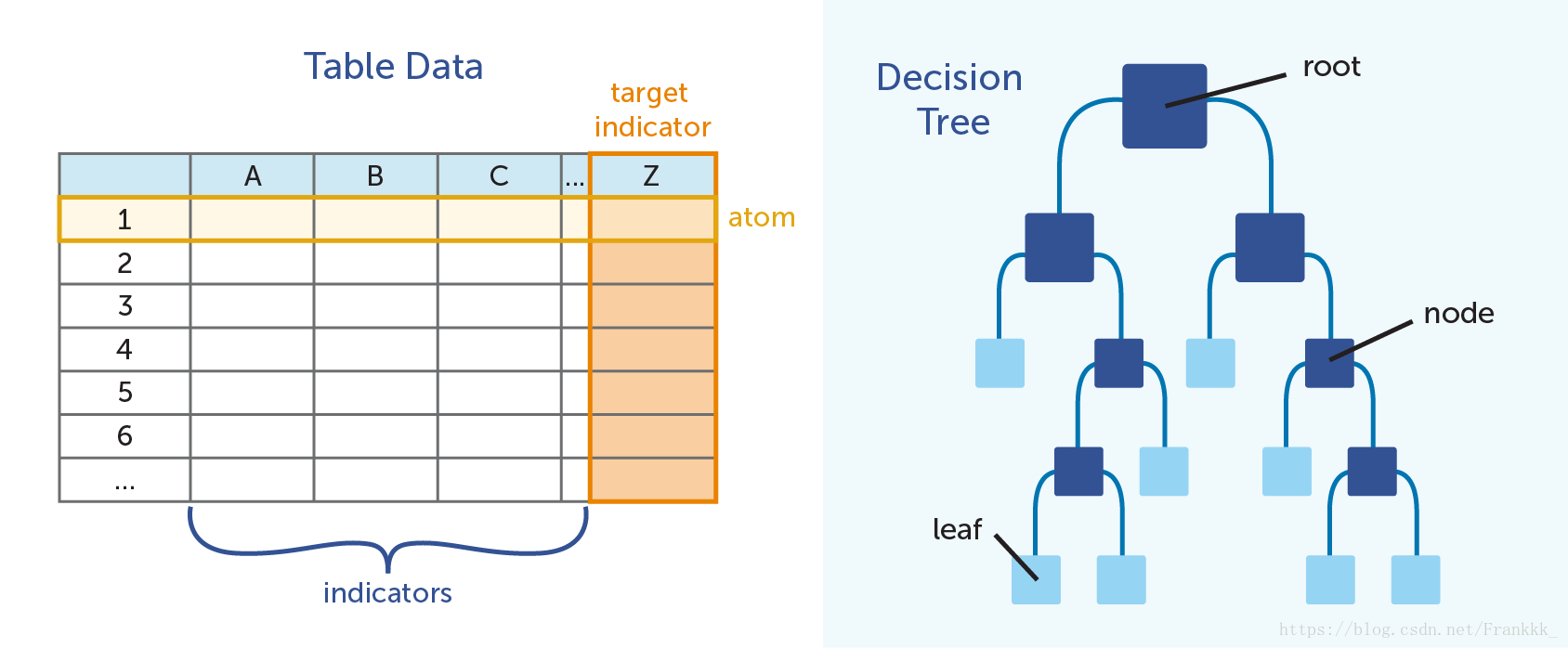
A decision tree for classification is a tree structure used to classify data. It mainly consists of nodes and directed edges. There are two types of nodes: internal nodes and leaf nodes. Internal nodes represent a feature or attribute, while leaf nodes represent a class. The structure is shown in the figure below:

1.2-Feature Selection

Feature selection involves choosing features that have classification ability for the training data, which can improve the learning efficiency of the decision tree. If the result of classifying using a feature is not much different from random classification, the feature is considered to have no classification ability. Discarding such features usually does not significantly affect the learning accuracy of the decision tree. The criteria for feature selection are typically information gain or information gain ratio.

In information theory, entropy is a measure of the uncertainty of a random variable. Let X be a discrete random variable with a finite number of values, and its probability distribution is:

$$P(X={ {x}_{i} })={ {p}_{i} },i=1,2,...,n$$

Then the entropy of the random variable is defined as:

$$H(X)=-\sum\limits_{i=1}^{n}{ { {p}_{i} }\log { {p}_{i} } }$$

The greater the entropy, the greater the uncertainty of the random variable. From the definition, it can be verified that:

$$0\le H(p)\le \log n$$

When $p=0$ or $p=1$, $H(p)=0$, indicating no uncertainty in the random variable. When $p=0.5$, $H(p)=1$, the entropy is at its maximum, indicating maximum uncertainty.

Conditional entropy $H(Y|X)$ represents the uncertainty of a random variable given the condition of another random variable. The conditional entropy of random variable $Y$ given random variable $X$ is defined as the mathematical expectation of the entropy of the conditional probability distribution of $Y$ given $X$:

$$H(Y|X)=\sum\limits_{i=1}^{n}{ { {p}_{i} }H(Y|X={ {x}_{i} })}$$

Here, ${ {p}_{i} }=P(X={ {x}_{i} }),i=1,2,...,n$. Information gain represents the degree to which the uncertainty of class $Y$ is reduced by knowing the information of feature $X$.

The information gain of feature $A$ on training set $D$, denoted as $g(D,A)$, is defined as the difference between the empirical entropy $H(D)$ of set $D$ and the empirical conditional entropy $H(D|A)$ of $D$ given feature $A$:

$$g(D|A)=H(D)-H(D|A)$$

1.3-ID3 Algorithm for Building Decision Trees

The main algorithms for decision trees are ID3, C4.5, and CART. The core of the ID3 algorithm is to apply the information gain criterion to select features at each node of the decision tree and recursively construct the decision tree. The ID3 algorithm for building a decision tree is as follows: Input: Training dataset D, feature set A, threshold $\varepsilon$; Output: Decision tree T.

1. If all instances in D belong to the same class ${ {C}_{k} }$, then T is a single-node tree, and ${ {C}_{k} }$ is used as the class label for this node. Return T.
2. If A is empty, then T is a single-node tree, and the class with the largest number of instances in D is used as the class label for this node. Return T.
3. Otherwise, calculate the information gain of each feature in A on D using the information gain algorithm, and select the feature ${ {A}_{g} }$ with the highest information gain.
4. If the information gain of ${ {A}_{g} }$ is less than the threshold $\varepsilon$, then T is a single-node tree, and the class with the largest number of instances in D is used as the class label for this node. Return T.
5. Otherwise, for each possible value ${ {a}_{i} }$ of ${ {A}_{g} }$, divide D into several non-empty subsets ${ {D}_{i} }$ based on ${ {A}_{g} }={ {a}_{i} }$. Use the class with the largest number of instances in ${ {D}_{i} }$ as the label to construct child nodes. The tree T is formed by the node and its child nodes. Return T. For the i-th child node, use ${ {D}_{i} }$ as the training set and $A-\{ { {A}_{g} }\}$ as the feature set, and recursively call steps 1-5 to obtain the subtree ${ {T}_{i} }$. Return ${ {T}\_{i} }$.

2-Ensemble Learning

Ensemble learning completes learning tasks by constructing and combining multiple learners. It is sometimes referred to as a multi-classifier system or committee-based learning.

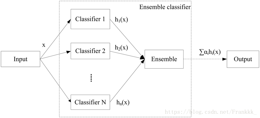
The figure below shows the general structure of ensemble learning: first, a set of “individual learners” is constructed, and then they are combined using a certain strategy. Individual learners are usually generated by an existing learning algorithm from training data, such as the ID3 decision tree algorithm, BP neural network algorithm, etc. In this case, the ensemble contains only the same type of individual learners, such as “decision tree ensemble” consisting entirely of decision trees, and “neural network ensemble” consisting entirely of neural networks. Such an ensemble is “homogeneous.” Individual learners in a homogeneous ensemble are also called “base learners,” and the corresponding learning algorithm is called the “base learning algorithm.” An ensemble can also contain different types of individual learners, such as both decision trees and neural networks. Such an ensemble is “heterogeneous.” Individual learners in a heterogeneous ensemble are generated by different learning algorithms, so there is no base learning algorithm; correspondingly, individual learners are generally not called base learners but are often referred to as “component learners” or simply individual learners.

By combining multiple learners, ensemble learning often achieves significantly superior generalization performance compared to a single learner. This is particularly evident for “weak learners,” and many theoretical studies on ensemble learning are targeted at weak learners. However, it is important to note that although using weak learners in an ensemble is theoretically sufficient to achieve good performance, in practice, for various reasons, such as wanting to use fewer individual learners or reusing some experience with common learners, people often use relatively strong learners.

Based on the generation method of individual learners, current ensemble learning methods can be roughly divided into two categories: serialized methods where individual learners have strong dependencies and must be generated serially, and parallelized methods where individual learners do not have strong dependencies and can be generated simultaneously. The representative of the former is Boosting, while the latter includes Bagging and “Random Forest.”

3-Random Forest Algorithm

Random Forest (RF) is an extended variant of Bagging. RF builds on the Bagging ensemble using decision trees as base learners and further introduces random attribute selection during the training process of decision trees. Specifically, traditional decision trees select the optimal attribute from the attribute set at the current node (assuming there are d attributes). In RF, for each node of the base decision tree, a subset containing k attributes is randomly selected from the attribute set at that node, and then the optimal attribute is selected from this subset for splitting. The parameter k controls the degree of randomness introduced: if k=d, the construction of the base decision tree is the same as a traditional decision tree; if k=1, a random attribute is selected for splitting; generally, the recommended value is $k={ {\log }_{2} }d$.

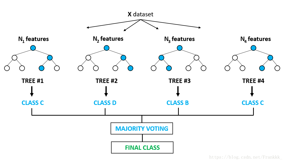
Random Forest is simple, easy to implement, and has low computational overhead. Surprisingly, it has shown strong performance in many real-world tasks and is praised as a “method representing the level of ensemble learning technology.” It can be seen that Random Forest makes only small modifications to Bagging, but unlike Bagging, where the diversity of base learners comes only from sample perturbation, in Random Forest, the diversity of base learners comes from both sample perturbation and attribute perturbation. This allows the generalization performance of the final ensemble to be further improved by increasing the diversity among individual learners. The structure of the decision tree is shown below:

For programming with Random Forest, you can use the scikit-learn framework: http://scikit-learn.org/stable/user_guide.html#