Compressing Neural Networks with the Hashing Trick

Abstract

As deep networks are increasingly applied to mobile devices, a dilemma becomes more apparent: the trend in deep learning is to develop models that can absorb larger datasets, yet mobile devices have limited storage space and cannot store overly large models. Here, a method called HashedNets is proposed to reduce model size by decreasing the inherent redundancy within neural networks. HashedNets use a low-overhead hash function to randomly group connection weights into different hash buckets, where all connections within the same bucket share the same parameter value, which is adjusted during standard backpropagation. This hashing process does not introduce additional memory overhead. Performance on various benchmark datasets indicates that HashedNets can significantly reduce storage requirements while preserving generalization performance.

1. Introduction

Over the past decade, deep neural networks have set new performance standards in many application areas, including object classification, speech recognition, image captioning, and domain adaptation. As data increases, the number of parameters in neural networks also grows to capture more information, often trained on industrial clusters and high-performance GPUs, which is a trend. Another trend is the migration of machine learning to mobile and embedded devices, which have relatively low power consumption and, importantly, only small working memory.

The separation between these two trends leads to a dilemma for state-of-the-art network applications on mobile devices. The most efficient models trained on industrial clusters may exceed the operational memory of mobile devices. One solution in the field of speech recognition is to send processed speech to a computing center for server-side computation, which requires high bandwidth. Another approach is to train small networks for mobile applications, but this sacrifices accuracy (as of 2018, this method is still feasible, partly because mobile computing power is growing rapidly, and lightweight networks like ShuffleNet perform well in terms of accuracy).

This dilemma has driven the development of network compression. Research shows that there is a lot of redundancy in neural networks, with only a small portion being useful, and has been explored using low-rank decomposition of weight matrices. Other studies have shown that deep networks can be compressed into shallow networks by training small networks using the outputs of fully trained networks (from the 2018 perspective, this is known as distillation, a term first proposed by Hinton in 2015, although related ideas appeared as early as 2006). There are also methods using reduced bit precision and methods proposed by LeCun in 1989 to remove unimportant weights from neural networks. In summary, many weight parameters in neural networks are unnecessary.

Numerous benchmarks demonstrate that HashedNets can significantly reduce model size with minimal impact on accuracy. Under the same memory constraints, the hashing method offers more adjustable parameters than low-rank decomposition. It is also found that reusing parameters under limited parameter sets is beneficial for expanding neural networks, and expanding HashedNets does not affect the design of other network structures (such as dropout regularization).

2. Feature Hashing

3. Notation

This section mainly introduces the symbolic representation of vectors, matrices, and the meanings of symbols in formulas.

4. HashedNets

This chapter introduces HashedNets, a variant of neural networks with significantly reduced model size and memory requirements. It first introduces the method of random weight sharing between network connections and then describes how to use the hashing trick to improve it, thus avoiding more memory overhead.

Fully connected network layers have many parameters. If there is a memory limit for each layer, and if it exceeds the memory limit, the memory occupied by each layer needs to be reduced. There are usually two methods: 1. Reduce the number of nodes in the connection. 2. Reduce the bit precision in the weight matrix. However, if the memory limit is already very small, these two methods will reduce the network’s generalization ability. A new method is proposed here: using a virtual weight matrix to reduce its effective memory consumption through weight sharing. The specific structure is shown in the figure: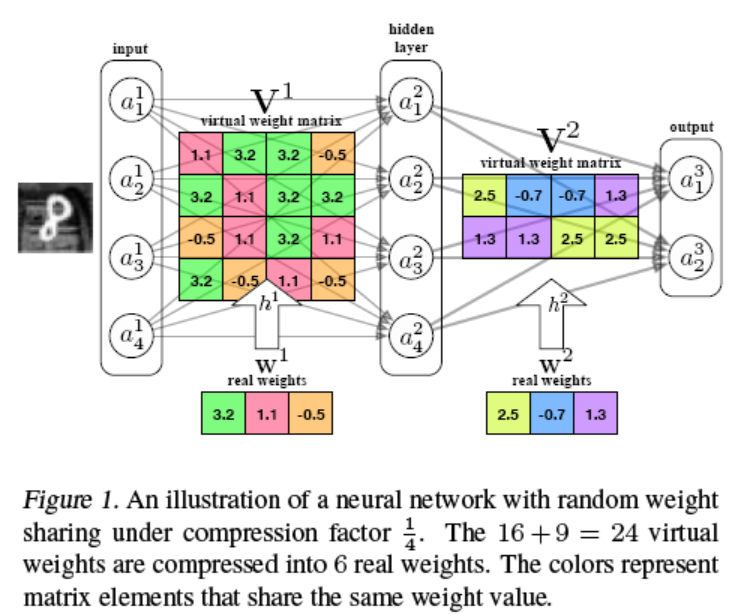

4.2. Hashed Neural Nets (HashedNets)

A simple implementation of random weight sharing is to use a second matrix to contain the grouping situation of each connection. However, such a detailed representation does not perform well in terms of memory savings. Here, hashing is used to achieve weight sharing, using $w^{l}_i$ to store the $i$ -th effective weight of the $l$ -th layer, $V^l_{i,j}$ represents the virtual weight, and a hash function $h^l(i,j)$ is used to map the indices on the virtual weight to the effective weight, i.e., $V^{l}_{ij}=w^{l}_{h^l(i,j)}$ . The open-source xxHash is used to implement this function.

The single-layer calculation formula of HashedNets is $z_i=\sum^{m}_{j=1}V_{ij}a_j=\sum^{m}_{j=1}w_{h(i,j)}a_j$ . HashedNets can also be interpreted through feature hashing, mapping the input m-dimensional features to k dimensions using hashing, achieving the same result as weight sharing, providing another explanation for HashedNets.

In feature hashing, the hash function is expressed as

[\phi_{i}(a)]_{k}=\sum_{j:h(i,j)=k}a_j

where $i$ represents the $i$ -th row in the weight matrix, $[\phi_{i}(a)]_{k}$ represents the $k$ -th element in the k-dimensional feature space after mapping. $z_i$ can be written as:

z_i=\sum_{k=1}^{K}w_{k}[\phi_{i}(a)]_{k}=\sum_{k=1}^{K}w_{k}\sum_{j:h(i,j)=k}a_j

Further transformation yields:

z_{i}=\sum^{m}_{j=1}\sum_{k=1}^{K}w_{k}a_{j}\delta_{[h(i,j)=k]}=\sum^{m}_{j=1}w_{h(i,j)a_{j}}

This expression is the same as the one obtained from weight sharing, indicating that the two are equivalent.

Sign factor: Due to the equivalence between random weight sharing and feature hashing, HashedNets inherit some advantages of feature hashing, such as eliminating inner product bias caused by conflicts by introducing $\xi(i,j)$ .

Sparsity: Previous research shows that applying feature hashing is most useful when the feature vector is sparse, as conflicts are smaller. Using sparsity-inducing activation functions in hidden layers can further promote this phenomenon, such as ReLU. Here, ReLU activation functions are used throughout due to their sparsity-inducing nature and strong generalization performance.

Alternative neural network architectures: This study mainly focuses on fully connected feedforward networks, but HashedNets can also be applied to other networks, such as RNNs, and can be combined with other network compression methods, such as using low-bit storage, removing certain edges, or training HashedNets using outputs from other large networks.

4.4. Training HashedNets

This section is divided into three parts: 1. Calculating the output of a hash layer during forward propagation. 2. Propagating gradients from the output layer to the input layer. 3. Calculating the gradient with respect to weights $W^l$ during backpropagation.

Forward propagation formula:

a_i^{l+1}=f(\sum^{n^l}_{j}w^{l}_{h^{l}(i,j)}\xi^{l}(i,j)a_{j}^l)

Error term:

\delta_{j}^{l}=(\sum_{i=1}^{n^{l+1}}\xi^{l}(i,j)w^{l}_{h^{l}(i,j)}\delta_{i}^{l+1})f'(z_{j}^l )

Gradient of the loss function with respect to parameters:

\frac{\partial L}{\partial V_{ij}^{l}}=a^{l}_{j}\delta_{i}^{l+1}\\ \frac{\partial V_{ij}^l}{\partial w_{k}^{l}}=\xi^{l}(i,j)\delta_{h^{l}(i,j)=k}

The first formula above is the derivative of the loss function with respect to virtual weights, and the latter is the derivative of virtual weights with respect to real weights. Using the chain rule to combine the two yields:

\frac{\partial L}{\partial w_{k}^{l}}=\sum_{i,j}\frac{\partial L}{\partial V_{ij}^l}\frac{\partial V_{ij}^{l}}{\partial w_{k}^{l}}=\sum_{i=1}^{n^{l+1}}\sum_{j}a_{j}^{l}\delta_{i}^{l+1}\xi^{l}(i,j)\delta_{h^{l}(i,j)=k}

Deep neural networks have made significant progress in many real-world applications, including image classification, object detection, image retrieval, speech recognition, and text expression. There have been many attempts to reduce the complexity of neural networks in various contexts. The most popular method is convolutional neural networks, which use the same filters in each receptive field, reducing model size and improving generalization performance. Combined with pooling, it can reduce connections between layers, only showing part of the input features. Autoencoders use the same weights between encoders and decoders.

Other methods can reduce the number of free parameters in the network but do not necessarily reduce memory overhead. One method for regularization is soft weight sharing, modeling weights as a mixture of Gaussian models: clustering weights so that weights in the same group have the same value. Since weights are not known before training, clustering is performed during training. This method differs from HashedNets, requiring many parameters to record the group membership of each weight value.

Another method is to directly remove unimportant weights, but this also requires many parameters to store sparse weight values. Experiments have shown that randomly removing connections in the network leads to good empirical performance, similar to the idea of HashedNets.

Some methods reduce model size by reducing numerical representation precision, such as 16-bit fixed-point representation, which reduces storage to 1/4 compared to double-precision floating-point representation, with only slight performance degradation. This method can be coupled with other methods.

Recent research shows that directly learning the low-rank decomposition of each layer reveals a lot of redundancy in neural network parameters. Networks recovered from low-rank decomposition only slightly degrade performance compared to treating all weight values as free parameters. Subsequent work uses similar techniques to accelerate CNN testing speed rather than reducing storage space and memory overhead. HashedNets complement this work, and the two methods can be combined.

Another method is distillation, where the authors show that distilled models have better generalization performance compared to training only on labels. A nested dropout method can rank the importance of hidden nodes, removing these nodes after training.

One method first proposed optimizing NLP models for mobile and embedded devices, using random feature mixing based on hash functions to group features, significantly reducing the number of features and parameters. With the help of feature hashing, the Vowpal Wabbit large-scale learning system can scale datasets.