Darts: Differentiable Architecture Search

Abstract

This paper aims to challenge architecture search by defining the task in a differentiable form, rather than the traditional approach of using reinforcement learning in a discrete, non-differentiable space. The method is based on a continuous relaxation of architecture representation, allowing for efficient architecture search using methods like gradient descent. Subsequent experiments show that the algorithm performs well in exploring high-performance CNN architectures for image recognition and RNN architectures for language modeling, and is much faster than existing state-of-the-art non-differentiable architectures.

1 Introduction

Automatically searched network architectures have achieved competitive performance in tasks like image classification and object detection. However, the best current architecture search algorithms demand significant computational resources. For example, using reinforcement learning to obtain a state-of-the-art architecture on CIFAR-10 and ImageNet requires 1800 GPU days. Some acceleration methods exist, such as setting specific structures for search space/weights/performance prediction and weight sharing across architectures. Yet, the fundamental scalability issue remains. The inefficiency of mainstream methods (RL, MCTS, SMBO, Bayesian optimization) stems from treating architecture search as a black-box optimization problem in a discrete space, necessitating numerous architecture evaluations.

This work proposes an alternative solution: DARTS (Differentiable Architecture Search), which relaxes the search space to make it continuous. This allows the architecture to be optimized using gradient descent, enabling DARTS to achieve performance competitive with state-of-the-art while requiring significantly less computation. The method also outperforms another efficient network search method (ENAS). DARTS is simpler than many other networks as it does not include any controllers/hypernetworks/performance predictors. Currently, DARTS performs well in searching both CNNs and RNNs.

The idea of conducting architecture search in continuous space is not new, but there are key differences here: previous work mainly focused on fine-tuning, such as filter shapes. DARTS can explore high-performance architectures in complex graph topologies with large search spaces and can be applied to both CNNs and RNNs. Experiments have shown that DARTS achieves excellent results on CIFAR-10, ImageNet, and PTB.

The main contributions of this paper can be summarized as follows:

1. Introduced a differentiable architecture search algorithm applicable to both CNNs and RNNs.
2. Demonstrated through experiments on image classification and language modeling that gradient-based architecture search achieves competitive results on CIFAR-10 and outperforms other state-of-the-art architectures on PTB. Interestingly, the best current architecture search algorithms use non-differentiable, RL, and evolution-based search techniques.
3. Achieved excellent architecture search efficiency using gradient-based optimization instead of non-differentiable search techniques.
4. The architectures learned by DARTS on CIFAR-10 and PTB can be transferred to ImageNet and WikiText-2.

2 Differentiable Architecture Search

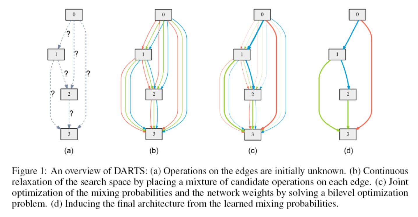
This section first provides an overview of the search space, describing the entire computation process as a directed acyclic graph. It then introduces the continuous relaxation of connections and the joint optimization of weights and architecture. Finally, an approximation technique is introduced to make computation feasible and efficient.

2.1 Search Space

The goal is to search for a computational cell to serve as the building block of the final architecture, which can be assembled into a CNN or connected into an RNN. A cell is a directed acyclic graph with N nodes, where each node $x^{(i)}$ represents a feature map, and each directed edge $(i,j)$ represents an operation $o^{(i,j)}$ that transforms $x^{(i)}$. Each node is computed from previous nodes:

$$x^{(i)}=\sum_{j<i}o^{(i,j)}(x^{(j)})$$

When there is no connection between two nodes, a null operation, denoted as the $zero$ operation, is introduced.

2.2 Continuous Relaxation and Optimization

Let $O$ be the set of all possible operations, each represented as $o(\cdot)$. To make the search space continuous, the selection of feasible operations is relaxed over all operations, similar to softmax:

$$\bar{o}^{(i,j)}(x)=\sum_{o\in O}\frac{exp(\alpha_{o}^{(i,j)})}{\sum_{o^{'}\in O}exp(\alpha_{o^{'}}^{(i,j)})}o(x)$$

The operation between two nodes $i,j$ is encoded as a $|O|$-dimensional vector $\alpha^{(i,j)}$. After relaxation, the task of searching the architecture becomes searching for a set $\alpha=\{\alpha^{(i,j)}\}$, which is also referred to as the encoding of the architecture. Finally, the mixed operation $\bar{o}^{(i,j)}$ is replaced by the most likely operation, for example, selecting the operation corresponding to the largest weight in the vector.

After relaxation, the next goal is to jointly optimize the weights $w$ and the architecture $\alpha$. Like RL and evolution, the accuracy on the validation set is used as a reward, but here gradient methods are used for optimization instead of searching in discrete space. Let $L_{train},L_{val}$ be the losses on the training and validation sets, respectively, determined by $w,\alpha$. This introduces a bilevel optimization problem:

$$min_{\alpha}\ L_{val}(w^{*}(\alpha),\alpha)\\ s.t. \ w^{*}(\alpha)=argmin_{w}\ L_{train}(w,\alpha)$$

Essentially, $\alpha$ can be viewed as a hyperparameter, albeit one with a dimension far greater than scalar hyperparameters.

2.3 Approximation

Solving such a bilevel optimization problem directly is challenging. Here, an approximate algorithm is provided:

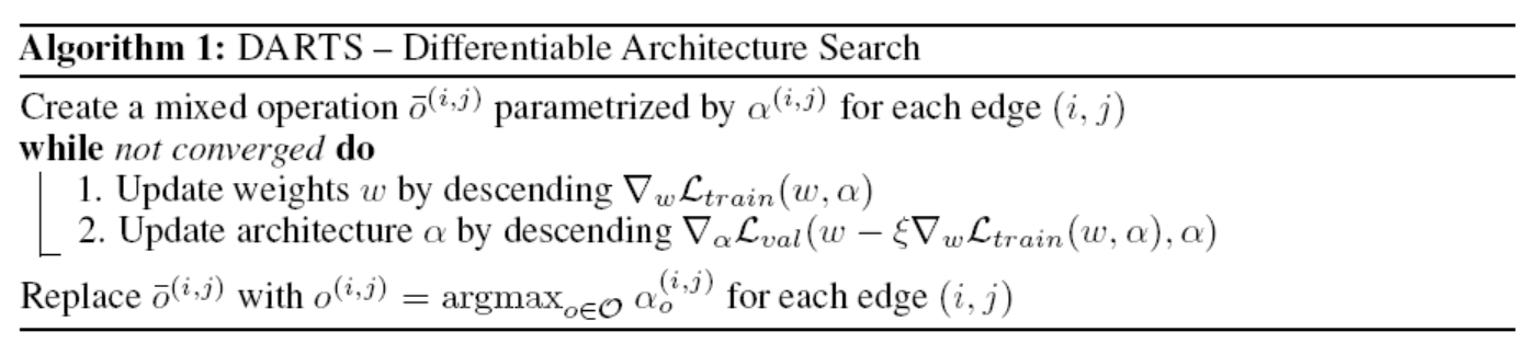
Essentially, it involves initially fixing the network architecture and optimizing the weights $w$, then optimizing the network architecture $\alpha$ based on the current weights, iterating back and forth until convergence. Finally, the mixed operation is determined as a specific operation. Note that in the above formula, when updating the network architecture $\alpha$, the term $w-\xi \nabla_{w}L_{train}(w,\alpha)$ is a single-step gradient descent to approximate $w^{*}(\alpha)$. A similar method is applied in model transfer meta-learning. This iterative algorithm defines a Stackelberg game between $w,\alpha$, although currently, there is no guarantee that the algorithm will converge. However, in practice, it can converge with a suitable choice of $\xi$. Also, note that when using momentum in weight optimization, the single-step forward algorithm will change accordingly, and the previous analysis remains useful.

In the first step, the gradient for $w$ is the normal backpropagation process in neural networks. In the second step, to update the network architecture $\alpha$, the gradient of $L_{val}(w-\xi\nabla_{w}L_{train}(w,\alpha),\alpha)$ with respect to $\alpha$ needs to be computed. It can be derived as:

$$\nabla_{\alpha}L_{val}(w-\xi\nabla_{w}L_{train}(w,\alpha),\alpha)=\nabla_{\alpha}L_{val}(w',\alpha)-\xi\nabla_{\alpha,w}^{2}L_{train}(w,\alpha)\nabla_{w'}L_{val}(w',\alpha)$$

where $w'=w-\xi\nabla_{w}L_{train}(w,\alpha)$ is the result after a single-step forward process. The latter term in the above formula involves a matrix-vector product, which requires significant computation. However, it can be approximated by a method where $\epsilon$ is a small quantity:

$$\nabla_{\alpha,w}^{2}L_{train}(w,\alpha)\nabla_{w'}L_{val}(w',\alpha)\thickapprox\frac{\nabla_{\alpha}L_{train}(w^{+},\alpha)-\nabla_{\alpha}L_{train}(w^{-},\alpha)}{2\epsilon}$$

where $w^{+}=w+\epsilon\nabla_{w'}L_{val}(w',\alpha),w^{-}=w-\epsilon\nabla_{w'}L_{val}(w',\alpha)$

This reduces the computational complexity from $O(|\alpha||w|)$ to $O(|\alpha|+|w|)$.

When $\xi=0$, the second-order term in the above formula becomes inactive, and the gradient of the loss function with respect to $\alpha$ becomes $\nabla_{\alpha}L_{val}(w,\alpha)$. This effectively removes the single-step propagation used to approximate the next $w$, which increases speed but results in poorer performance. The case where $\xi=0$ is referred to as first-order approximation, while $\xi>0$ is referred to as second-order approximation.

2.4 Deriving Discrete Architectures

After training, it is necessary to generate the corresponding discrete architecture. First, select the k strongest predecessors for each intermediate node. Here, for CNNs, k=2, and for RNNs, k=1. The strength of an edge is defined as: $max_{o\in O,o\neq zero}\frac{exp(\alpha_{o}^{(i,j)})}{\sum_{o'\in O}exp(\alpha_{o'}^{(i,j)})}$

Then, each mixed operation is determined as a specific operation by selecting the most likely value.

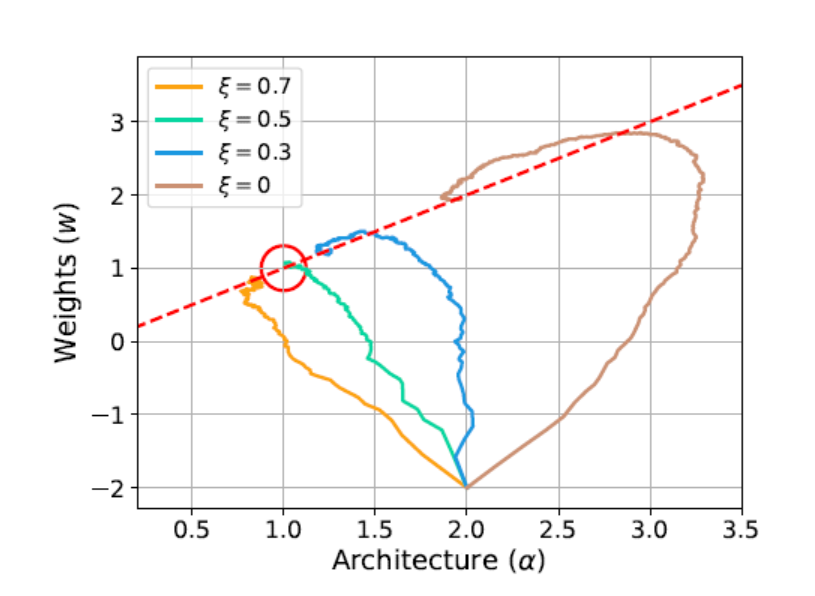
The convergence path obtained from experiments under a simple L_val and L_train is shown below. Comparing with the analytical solution of the problem, the iterative algorithm can converge to a better result with the correct choice of $\xi$.

3. Experiments and Results

Experiments conducted on CIFAR-10 and PTB involve two stages: architecture search and architecture evaluation. In the first stage, possible cells are searched, and the best set of cells is determined based on performance on the validation set. In the second stage, these cells are used to build larger networks, and their performance is reported on the test set. Finally, the transferability of the best cells is evaluated. This summary primarily covers the CNN-related parts, excluding the RNN content.

3.1 Architecture Search

This section summarizes the convolution-related parts. The operation set includes $O$: 3x3 and 5x5 separable conv, 3x3 and 5x5 dilated separable conv, 3x3 max pooling, 3x3 avg pooling, identity, zero. All operations have stride=1, and convolution operations use the ReLU-Conv-BN sequence, with each separable conv applied twice.

The conv cell includes 7 nodes, with the output node defined as the depthwise concat of internal nodes. The first and second nodes in cell k are equal to the outputs of cell k-1 and cell k-2, using 1x1 conv when necessary. Cells in the 1/3 and 2/3 parts of the network are reduction cells, where all operations connected to input nodes have stride=2. Thus, the architecture encoding is divided into $\alpha_{normal},\alpha_{reduce}$.

During the entire search process, the architecture changes, using batch-specific statistics instead of global moving averages in BN, and disabling learnable affine parameters in all BNs.

Half of the CIFAR-10 training data is used as the validation set, training a cell=8, 50 epochs, batch_size=64, initial_channels=16. These parameter settings ensure training on a single GPU. The optimization of w uses momentum SGD, and the optimization of $\alpha$ uses Adam, taking a total of one day on a single GPU.

3.2 Architecture Evaluation

To select the architecture for evaluation, DARTS was run four times with different random seeds, and the best cell was selected based on validation set performance. The weights were then randomly initialized and trained again to observe performance on the test set.

After selecting the cell with a small network, a larger network is trained with 20 cells, 600 epochs, batch_size=96, and some other enhancements: cutout, path dropout, auxiliary towers. Training took 1.5 days on a single GPU.

3.3 Results Analysis

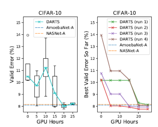
The experimental results of DARTS on CIFAR-10 and ImageNet are shown below. The same cells as CIFAR-10 were used on ImageNet:

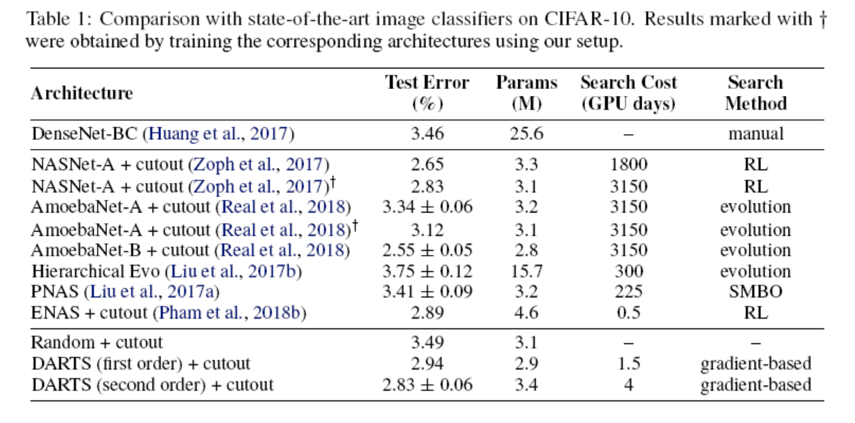
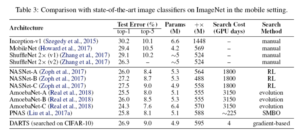
In the above figures, NASNet and AmoebaNet are state-of-the-art. In comparison, the performance difference is small, but the search time is significantly reduced. The same effect is observed for the ImageNet dataset.

4. Conclusion

DARTS is the first differentiable architecture search algorithm applicable to both CNNs and RNNs. By searching in continuous space, DARTS can match or even outperform state-of-the-art non-differentiable architecture search algorithms in image classification and language modeling tasks, and is significantly more efficient. In the future, DARTS will be used to explore direct architecture search on larger tasks.